Latent Space Phenotyping #3
Mar 13, 2020
Hello dear reader,
There might be enough readers to actaully make this exercise worth it! No one will ever know… unless you comment in the comment box. Dr. Amy Tabb (@amy_tabb) commented once and that was pretty cool, because now at least I am sure the function works! Hizzah!
Random endorsement: If you are stuggling, like I was, with writing. I can highly recommend using OverLeaf. Their nice UI to LaTeX made preparing a very clean and “pre”-formatted manuscript a lot of fun and very simple. Even my PI likes it! The compiler actually made the process feel like I was making progress towards a real product. Several students in the Knapp lab have started using OverLeaf and seem to love it, as well. LOVE it. This is unsponsored content, but I am down with sponsored content too. wink wink hint hint
This round I am going to wax and wane poetically on my own work: Feldmann et al. (2020) “Multi-Dimensional Machine Learning Approaches for Fruit Shape Phenotyping in Strawberry” Accepted to GigaScience. However, I am still waiting on authorproofs.
For now, you can find the original submission here: https://doi.org/10.1101/736397 and I will update this post once the final manuscript is available on GigaScience.
This paper, and its yet written siblings, go back to my first year as a graduate student at UC Davis (2015). I was left mostly to my own devices, I was really excited to be a PhD student, and I fixated on morphometrics and multivariate statistics. For this, I blame Dr. Chitwood and his 2014 PLoS One paper on the temporal variation of violin shape (https://doi.org/10.1371/journal.pone.0109229). Read it. Love it. Be as inspired as I was. It is fun. It is cool. It is genuinely good. The figures are beautiful. The writing is beautiful. I then became aware of the on going work in tomato, grape, and Passiflora leaves (https://doi.org/10.1093/gigascience/giw008) and I was caught… hook, line, and sinker…
Thanks, Dan.
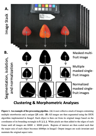
My thesis focuses on yield in strawberry, but I also inherited the weight of fruit quality assessments (Brix, Acidity, Anthocyanins, Texture, color, etc). These assessments are incredibly expensive, and so in order to get the most out of it, I took images containing >2 strawberries on average (1-3) (Figure 1) with the intent of doing Elliptical Fourier analysis and some linear descriptors (aspect ratio, circularity, etc.). The basics, I guess.
As I started learning how to extract features, I became… inspired.
TLDR; I extract 68 continuous features from each image using classic methods and novel methods. Please jump ahead 5 paragraphs to continue.
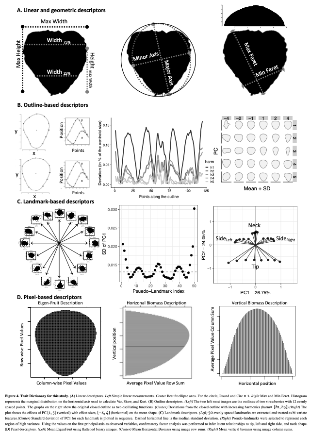
(1) I extracted 11 linear/geometric features. These primarily came out of ImageJ, which I used for segmenting and isolating individual fruit, and consist entirely of ratios that are scale invariant.
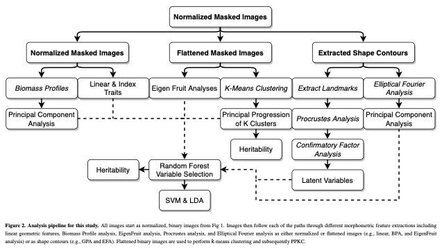
(2) I performed Elliptical Fourier analysis with 5 harmonics resulting in 20 coefficients. Typically, PCA is performed on these coefficients to try to summarize as much of the total variance on as few independent axes as possible. Honestly, I forgot to use only the PCs that explained ~90-95% of the variance and all 20 PCs made it into Figure 5. Somehow, no one caught this. It isn’t really important, but it is a little sloppy of me.
(3) Dr. Sarah Turner-Hissong had a really cool paper on carrot organ shapes (https://doi.org/10.3389/fpls.2018.01703), that I drew inspiration from. Effectively, they transform each image into a vector of rowSums and then do PCA on the matrix that is n_images x n_rows/image.
(4) The, I flattened each image and did PCA on the whole damn set of 10,000 pixels. I was using 6,874 images so this returned 6,873 non 0 PCs. It required ~220 of these to describe 90% of the data… I kept 20, because that explained 75% of the variance… This method is exactly the PC approach that Gage et al 2019 (doi:10.2135/tppj2019.07.0011) took to describe the plot level heat maps. I suppose I could have done an auto-encoder network too, but… I didn’t.
(5) Strawberry outlines do not have obvious, biologically homologous landmarks (like grape/tomato leaves). To be able to perform generalized procrustes analysis, I broke the outline of each shape into a set of 50 evenly spaced pseudo-landmarks. I decomposed each landmark using PCA. and discarded landmarks with major axis variance less than the median major axis varianceof all landmarks. There was greater landmark variance at the tip and neck, as well as the left and right side of the fruit (the polar coordinates). These more variable landmarks were selected and then treated as observed variables in a SEM with 5 latent variables. 4 of these were manifest directly from the observed variables (i.e., they represent the “shared” variance of the observed variables) in the tip, neck, and the two side regions. The last latent variable is manifest by the 4 previous latent variables, and represents the shared variation of those 4 latent variables. I called this last variable “Shape.” I had not seen this approach taken before, and at the time I was really excited about SEM, so much so that I took a class on SEM, taught by Dr. Mijke Rhemtulla, in my 5th year at UCD.
At this point I had too many variables (68) and honestly, that was both frightening and exciting. The entire goal was quantitative genetic analyses, but how on earth do you make sense of 68+ correlated traits that describe a single trait, i.e., fruit shape? Machine Learning.
TLDR; I use k-means cluster to classify images based on the pixel values (only 4 classes matter), random forest regression for variable selection (only 5 variables matter), and support vector machines on a reduced set of features from classification. Classification at the target level, with a reduced set of features works really well. Please skip the next three paragraphs.
(1) I needed to be able to classify ~7,000 fruit in a rapid and repeatable what. K-means was the chosen algorithm, primarily because it is reasonable fast and very easy to implement in R, you can perform classification multiple times to test reliability, you can do CV, you can get goodness-of-fit metrics, and because there was no way in hell that I was going to classify 7,000 images (I envisioned using Amazon M-Turks for this task early on). The goodness-of-fit metrics allows us to determine that there are 4 primary shape categories in UCD strawberry germplasm, which is great because the other options in the strawberry community consist of 9 unit ordinal scales. The more categories you have the worse any human is going to be at classifying a shape and the more exhausting the task becomes, IMO. I think that there is some nice work that demonstrates this as well (https://doi.org/10.1371/journal.pcbi.1006337).
(2) I performed variable selection using random forest regression. There is a wonderful R package for this called “VSURF” that made variable selection really stinking easy. I performed RF classification for each value of K (i.e., 2-10) and selected the variables that were most important in 3/9 values of K. The reasoning behind this is that I want to only choose features that would be broadly predictive of shape class across multiple levels of K. In a more targeted approach, I would have selected only those variables that were most important for delineating the K=4 primary clusters.
(3) Then, I performed Support Vector Classification and Linear Discriminant Analysis using e1071::svm() and MASS::lda(). I chose these two algorithms because they are widely known. I had considering also doing quadratic discriminant analysis, but I figure that it would land somewhere in between svm and lda anyways. Could be a cool extra bit for a tutorial later on? Accuracy of classification was surprising to me (in a good way). I will let you check out the last table in the paper, it is a doozy and goes on forever, I apologize. There were so many facets, and I didn’t know how else to summarize it all.

All in all, very few descriptors were needs to obtain high classification accuracies beyond the fit of k-means. The heritability of the predictors was high as well.
I really loved working on this project, I have a ton of ideas for the next steps plus another year of images to analyze, and I have 50K genome-wide SNPs. Now I am staring down the barrel of super fun multivariate prediction and GWAS experiments. Beyond that, I would really like to explore sparse factor models for this type of image data. The final image data set is going to be ~14,000 x 10,000 with tons of strong correlations, so I think a sparse factor model ,like Dr. Dan Runcie’s BSFG, would be really fun to apply here.
This work is hard to sell. It is 2D which is not holistically descriptive of strawberry fruit shape. It is is exclusively shape, which is not what most consumers are focused on, and most breeders and packers would be more concerns with ship-ability rather than “shape.” But shape is part of appearance and is also part of packability and ship-ability. There is a lot of work to make fruit shape a critical component of strawberry breeding. We probably need to find the yield ceiling first.
One idea I had, was to ask my twitter feed (and their twitter feeds) to participate in an online survey for fruit shape preference, to understand what the preferred shape is. It became clear, after discussion with Michaela DeBolt (@MdeboltC) that I have no idea how to design a proper survey that will lead to unbiased answers, and so I dropped it. That, plus the requisite IRB approval, basically stopped me in my tracks on that front
The future of this work is unknown and tightly linked to present status of latent space phenotyping and morphometrics. I desperately hope to do more work like this in the future, because it is fun, challenging, motiviating, creative, and as infinite as our resolution and resolve.
Best, Mitchell
PS. I realized after posting this that I had forgotten to talk about PPKC, which I will save for the next post.