Latent Space Phenotyping #2
Feb 25, 2020
Hello dear reader,
I will probably never have more than one reader (Hi mom!) on these blog posts, but that is ok. This has already proven to be an entertaining method of being productive when other things are moving slower than they should (reviews on manuscripts, genotyping samples, etc.).
I have decided, this week, to stick with the Latent Space Phenotyping theme because I find the topic endlessly amusing and constantly engaging. The manuscript of interest is Gage et al (2019) “In‐Field Whole‐Plant Maize Architecture Characterized by Subcanopy Rovers and Latent Space Phenotyping”. https://doi.org/10.2135/tppj2019.07.0011
Again, I was lucky to talk with Joe Gage, PhD during a recent visit to Ithaca about this work. That was one of the best phenotyping conversations I have had in a long time, and it was so memorable and exciting because of the similarity in the methods that Joe and I had landed on for analyzing images. My own work was recently accepted in GigaScience.
You will also notice, maybe, that the authors cite Ubbens et al (2019) throughout their introduction (7x) (it is an awesome paper IMO). Because of this, I am not going spend much time talking about the coolness of using auto-encoders and dimension reduction techniques to summarize massively multivariate data sets (e.g., a 100x100 image has 10,000 correlated features). Now imagine you are dealing with 3D data or image cubes (e.g., hyper-spectral data). The number of correlated features becomes GIGANTIC. So, researchers need to be creative in how to handle and utilize such data. Could you project any 3-D point cloud or model onto a plane and make genetic sense of it?
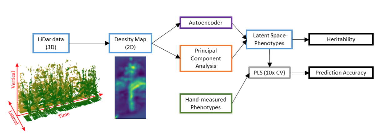
This is what I find so exciting about this paper. The author’s collected 3-D LiDar data of maize plots from the back of a terrestial rover. LiDars are fast rotating sensors that are commonly used in plant phenotyping, but also engineering and architecture, to get accurate depth and distance information. These can be controlled with a Raspberry Pi (https://learn.adafruit.com/slamtec-rplidar-on-pi/360-degree-lidar) and are inexensively deployed. I have been personally considering purchasing one, just to learn how to explore the data.
The Rover with the LiDar drives through the 2-row plots collecting data on every plant that it passes, giving a 3D point cloud reconstruction of the plot. I think the authors drove the rover on each side of the plot and through the middle for this project. Each point cloud of each plot was then transformed into a 2-D heat map by collapsing the 3D reconstruction along the time axis. Each heat map summarized an entire plot (entry) and each pixel in that heat map indicates the number of points observed at that height through the entire plot. Instead of attempting to reconstruct individual plants and average across each poorly isolated plant, the authors wisely chose to average across everything and ignore the plant-level phenotypes. Each experimental unit is represented as a single matrix that can be flattened and analyzed using PCA, an ANN, or both, as done here.
I think now may be the appropriate time to really start talking about my biggest struggle with LSP. Broadly, this concern can be summed up as, “so what?” There is so much room for creative thinking on the analytical side, but we absolutely need be able to link the image features to “real-world” plant phenotypes and measurement that actually matter in the agricultural complex and that can be used to make faster, less expensive, more effective selection decisions.
The first thing that the authors do towards this goal is to estimate the broad-sense heritability of their extracted PC/ANN features alongside a suite of 12 manually measured traits (Fig 5). The PCs and ANN feature are moderately heritable (0.44 >= H2 >= 0.0). Correct, the broad sense of some of the PC features have 0 heritability, despite explaining some reasonable amount of image variance, I assume. H2=0 effectively means that the genetic variance is perfectly orthogonal to error variance. In other words, there is phenotypic variance but none of it can be attributed to intra-class differences. I would like to see these features dropped from subsequent analyses since they are attributable to random design effects, and not treatments (entries). The highest heritability is in the upper two PCs, which makes sense as they should be describing the most “salient” / highest variance features of the images. However, PC4 has a very low heritability. I have noticed a trend in this kind of data and image-based analyses that results in leading PCs having nearly 0, or 0, heritability. This phenomenon is observed in other morphometric analyses, although it may be more common in analyses that don’t performing smoothing (noise reduction) prior to feature extraction (e.g., PCA). How big of a challenge is noise in image based phenotyping to be such a large, even dominant, feature in these analyses?
The second thing these authors do to attempt to make sense of these LSPs is predict classic hand measured traits (e.g., plant height) using either the PC or the ANN embeddings using Partial Least Squares Regression. In general, both methods perform about the same across the different hand measured traits. So, which analysis, or set of LSPs, is preferred? This is a truly philosophical debate that has no answer. The PCA approach is a rotation of the data that maximized the independent (orthogonal) variance on each axis, while the ANN can be made of both linear and nonlinear embeddings. PCA is very easy to run and ANNs are a bit trickier and take a bit more finesse (I personally have run into all of the possible issues getting different ML front and backends installed; versions, dependencies, folders nested too deep, files not found… you name it). Both are equally heritable. Both are equally predictive. Why not stick with the PC based approach? I think the authors do a great job with a really interesting type of data (Rover mounted LiDar) that I personally haven’t seen before and they do a great job describing and making their work available.

The authors discuss the cost of deploying a rover vs the cost of deploying humans for phenotyping (the rover is much cheaper) and the prediction of certain traits is quite high. But is it high enough to convince a more “traditional” agronomist or breeder to adopt a new method? One thing I would like to see, and this goes for most ag focused phenomic work, is a coincidence score of the top 10% plant height against the top 10% LSP predicted plant height, or what ever traits the LSPs are proxy for. I were to select based on the LSP prediction, am I going to be discarding and keeping the same lines as if I were to select on hand measurements? What is the difference in genetic gain made by acting directly on plant height or through a correlated LSP? This, at least, would make for a valuable follow up and I recognize that not all problems can/should be tackled in a single document.
I, for one, am excited for the continued integration of terrestrial and aerial unaccompanied automous vehicles (UAVs) into phenomics, genetics, and agriculture.
Best, Mitchell
PS. As my own work starts to hit the shelves, I will probably do a break down of that material in this blog.