Latent Space Phenotyping
Feb 18, 2020
Hello dear reader,
I am thinking about adopting a paper review style format for this blog. This may extend to albums as I expand the old list of things that I am currently listening to and currently reading, see the homepage. Also, I should mention that my style will likely be a bit “from the hip.”
That being stated, I am going to start with Ubbens et al (2020) Latent Space Phenotyping: Automatic Image-Based Phenotyping for Treatment Studies. https://doi.org/10.34133/2020/5801869.
I was able to talk about this work with Jordan Ubbens (@jordanubbens) at Phenome 2019 after his presentation on this work, because he replied to a Twitter message. I slipped into his DMs so-to-speak. IFF you are attending Phenome2020, I highly recommend the digital phenotyping workshop that Jordan is speaking at.
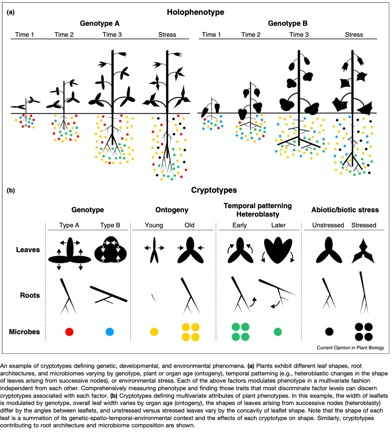
Anyways, I find this work fascinating because it is closely related to several projects that I am working on regarding fruit shape. Furthermore, there has recently been more references to “latent space phenotypes” (LSP) and as far as I can tell, that stems from this paper. At least it is the reference that Joseph Gage and I have used for this phrase. However, it is of the same conceptual meaning as a “Cryptotype” coined by Dr. Daniel Chitwood and Dr. Christopher Topp. “We propose the term cryptotype to describe latent, multivariate phenotypes that maximize the separation of a priori classes” (Chitwood & Topp 2015). This idea of a latent space extends back to the 80s with Eigen-faces, which was used in plants by Horgan in the early 2000s to examine internal color variation in carrots.
What is a LSP? In this manuscript, Ubbens defined LSPs as “a broad family of techniques known as latent variable models […] LSP instead constructs a latent representation that best discriminates between image sequences of control and treated samples of a plant population and then measures differences among individuals within the latent space to quantify […] the effect of the treatment. The key characteristic of LSP in comparison to existing image-based phenotyping methods is that the phenotype estimated using an image analysis pipeline is replaced with an abstract learned concept […] inferred automatically from the image data using deep learning techniques.”
What this means is that LSPs don’t have the same type of direct interpretation as height or width and thus they are challenging to describe outside of the context of the sample and its relationship to all other samples. So, an LSP is any number or set of numbers that can be extracted from an image through any set of techniques. One interpretation of an image that makes the most sense in image-based phenotyping is that the image is simply a matrix of numbers, and we want describe the relationship between the values in that matrix. This is not a new interpretation, but reaching it really helped me recognize the huge value in getting high quality images with as little noise as possible as LSPs are first and foremost going to describe the most salient aspects of that image (e.g., those aspects that explain the most variance)
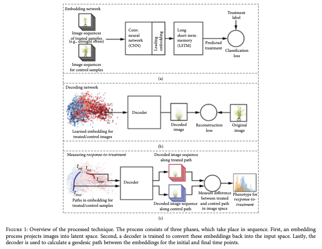
This is why I enjoy this paper so much. The authors use longitudinal treatment-control experiments and encode a reduced space using a encode-decoder CNN. This type of network effectively projects a matrix so a much smaller parameter space and then attempts to decode that reduced space to reconstruct the original image. The goal is to minimize a loss function while maintaining accuracy in the decoding network (you want your encoding to represent your image uniquely) and using an appropriate number of neurons in your encoded representation. It doesn’t help much, from a quantitative genetics perspective, to drop from 10,000 to 1,000 parameters, but 10,000 to 10 becomes actionable and tractable for GWAS/GS, albeit a little confusing.
However, the authors took a very interesting approach which allowed them to potentially maintain quite a few parameters in their encoded layer (I did not dig too deeply into their python scripts for this, but honestly I should). The approach they took was to estimate the geodesic distance from starting point to end point in their longitudinal data for both treated plants and control plants. The geodesic distance is a good choice because it is forced to follow defined path through points (with 6 time points, there would be 5 paths) and each of 6 nodes would have some linear distance in multidimensional space to the subsequent node. The geodesic distance is then the sum of all of the relevant path lengths and is a single value(!). Brilliant. These two paths (one for the treatment and one for the control) can then be compared directly as an estimate of the difference between the plant growth habits in the treatment and control conditions. BRILLIANT! This is common practice in nutrient deficiency studies, but instead of extracting some variable from the image (e.g., plant size) the entirety of the image dictates what gets analyzed. In this manuscript, the authors re-analyze a published data set on Setaria (discovered overlapping results!!) and also analyzed some simulated data sets.
A pitfall of this type of analysis is noise in the images. If the object of interest isn’t the most salient feature in your image you have to jump through a bunch of pre-processing hoops to force it to be the most salient feature (e.g., background extraction, segmentation, etc.). Dr. Larry York came up with a really clever design for the RhizoVision Crown system, which puts a light box behind the object of interest. Using a grayscale camera, the images are segmentated binary maps from the start. This approach works well with roots and would likely work with plants and fruit as well. However, its a no-go if you are interested in color, even relatively speaking. Excitingly, the approach used by Ubbens can also potentially handle RGB and hypers-pectral layers as well, although I don’t recall if they do in this manuscript.
The other challenge is simply owning the proper computing machinery. Neural Networks are notoriously data hungry and expensive to run. Speedups with GPUs are good to reduce the time cost, but powerful GPUs don’t tend to be the most power efficient devices (better than more CPU cores though). The size of the network is driven by the number of input values, the number of layers, and the neurons in each layer. These typically need to be user defined, which means to get the best results (time, loss, and accuracy), multiple networks need to be initialized and compared before settling down on the preferred network.
I have recently become aware of some relatively lightweight R packages for auto-encoders. It may be a fun exercise to do a side by side comparison with Keras/Tensorflow and R/autoencoder and R/ANN2.
Best, Mitchell